Modelling the Kobayashi Benchmark Problems
In this tutorial, you will learn how to model more complicated 3D fixed source problems in Kobayashi et al. (2001) with Gnat. To access this tutorial,
cd gnat/tutorials/3D_kobayashi
Common Material Properties
All of the Kobayashi problems use the same material properties. These consist of an isotropic neutron source, a near-void material (to generate streaming paths), and a shield. The specifications for the materials can be found in Table 1.
Table 1: Material properties for the Kobayashi benchmarks.
| Material | () | () | () |
|---|---|---|---|
| Source | 1.0 | ||
| Near-Void | 0.0 | ||
| Shield | 0.0 |
Volume Source in a Cubic Shield
The first Kobayashi benchmark problem consists of a cubic volume source with one corner centered on the origin. The source is surrounded on three sides by a thick near-source reigon, which is further encased in a thick shield. The boundary planes with , , and use reflective boundary conditions. The boundary planes with , , and are vaccum boundaries. The geometry of the problem can be found in Figure 1.
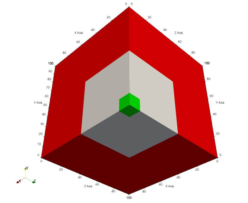
Figure 1: Geometry of the first Kobayashi problem. Green: source. White: near-void. Red: shield.
The Gnat input file to model this problem starts with the mesh, which is generated with a CartesianMeshGenerator. We specify that the generated mesh should be 3D (dim = 3) and that we have three distinct subdivisions with dx, dy, and dz. We then set the number of elements we want for each subdivision with ix, iy, and iz. In this model, we start with one element per interval. We then add block ids for material and volume source assignment using subdomain_id. This vector must be the same length as the product of the lengths of dx, dy, and dz. The generated mesh is uniformely refined once with uniform_refine = 1. This mesh generator automatically adds side sets for the six faces of the cube named left, right, top, bottom, front, and back which we can use for boundary conditions.
[Mesh]
  [domain]
    type = CartesianMeshGenerator<<<{"description": "This CartesianMeshGenerator creates a non-uniform Cartesian mesh."}>>>
    dim<<<{"description": "The dimension of the mesh to be generated"}>>> = 3
    dx<<<{"description": "Intervals in the X direction"}>>> = '10 40 50'
    dy<<<{"description": "Intervals in the Y direction (required when dim>1 otherwise ignored)"}>>> = '10 40 50'
    dz<<<{"description": "Intervals in the Z direction (required when dim>2 otherwise ignored)"}>>> = '10 40 50'
    ix<<<{"description": "Number of grids in all intervals in the X direction (default to all one)"}>>> = '1 4 5'
    iy<<<{"description": "Number of grids in all intervals in the Y direction (default to all one)"}>>> = '1 4 5'
    iz<<<{"description": "Number of grids in all intervals in the Z direction (default to all one)"}>>> = '1 4 5'
    subdomain_id<<<{"description": "Block IDs (default to all zero)"}>>> = '
    2 0 1
    0 0 1
    1 1 1

    0 0 1
    0 0 1
    1 1 1

    1 1 1
    1 1 1
    1 1 1'
  []
  uniform_refine<<<{"description": "Specify the level of uniform refinement applied to the initial mesh"}>>> = 1
[]After specifying the mesh, we move on to setting up the transport system. The Kobayashi problems are mono-energetic, so we specify that we only want a single energy group. Similarily, the scattering cross sections are isotropic and so we don't need to evaluate higher order angular moments of the flux. We specify that we want to use the SAAF-CFEM-S method with scheme = saaf_cfem, and that particle_type = neutron (which is arbitrary, particle_type = photon would also suffice). We specify that linear Lagrange basis functions should be used, and that a Gauss-Chebyshev angular quadrature set with five polar angles and five azimuthal angles per octant of the unit sphere should be used. Finally, we apply reflective boundary conditions along the lines of symmetry, apply vacuum boundary conditions to the remaining faces, and specify that the isotropic volume source with unit intensity should be applied to block 2.
[TransportSystems<<<{"href": "../syntax/TransportSystems/index.html"}>>>]
  [Neutron]
    num_groups<<<{"description": "The number of spectral energy groups in the problem."}>>> = 1
    max_anisotropy<<<{"description": "The maximum degree of anisotropy to evaluate. Defaults to 0 for isotropic scattering."}>>> = 0
    scheme<<<{"description": "The discretization and stabilization scheme for the transport equation."}>>> = saaf_cfem
    particle_type<<<{"description": "The type of particle to be consuming material property data."}>>> = neutron

    order<<<{"description": "Specifies the order of the FE shape function to use for this variable (additional orders not listed are allowed)."}>>> = FIRST
    family<<<{"description": "Specifies the family of FE shape functions to use for this variable."}>>> = LAGRANGE

    n_azimuthal<<<{"description": "Number of Chebyshev azimuthal quadrature points in a single octant of the unit sphere. Defaults to 3."}>>> = 5
    n_polar<<<{"description": "Number of Legendre polar quadrature points in a single octant of the unit sphere. Defaults to 3."}>>> = 5

    vacuum_boundaries<<<{"description": "The boundaries to apply vacuum boundary conditions."}>>> = 'right top front'
    reflective_boundaries<<<{"description": "The boundaries to apply reflective boundary conditions."}>>> = 'back bottom left'

    volumetric_source_blocks<<<{"description": "The list of blocks (ids or names) that host a volumetric source."}>>> = '2'
    volumetric_source_moments<<<{"description": "A double vector containing a list of external source moments for all volumetric particle sources. The external vector should correspond with the order of 'volumetric_source_blocks'."}>>> = '1.0'
    volumetric_source_anisotropies<<<{"description": "The anisotropies of the volumetric sources. The vector should correspond with the order of 'volumetric_source_blocks'"}>>> = '0'
  []
[]Next, the material properties of the domain must be specified with TransportMaterials:
[TransportMaterials<<<{"href": "../syntax/TransportMaterials/index.html"}>>>]
  [Shield]
    type = ConstantTransportMaterial<<<{"description": "Provides the particle group velocity ($v_{g}$), particle group total cross-section ($\\Sigma_{a,g}$), and the scattering cross-section moments ($\\Sigma_{s, g', g, l}$) for transport problems. If no scattering cross-section moments are provided, the material initializes all moments to 0. The properties must be listed in decreasing order by energy.", "href": "../source/materials/ConstantTransportMaterial.html"}>>>
    transport_system<<<{"description": "Name of the transport system which will consume the provided material properties. If one is not provided the first transport system will be used."}>>> = 'Neutron'
    group_total<<<{"description": "The macroscopic particle total cross-sections for all energy groups."}>>> = '0.1'
    group_scattering<<<{"description": "The group-to-group scattering cross-section moments for all energy groups."}>>> = '0.05'
    anisotropy<<<{"description": "The scattering anisotropy of the medium."}>>> = 0
    block<<<{"description": "The list of blocks (ids or names) that this object will be applied"}>>> = '1 2'
  []
  [Duct]
    type = ConstantTransportMaterial<<<{"description": "Provides the particle group velocity ($v_{g}$), particle group total cross-section ($\\Sigma_{a,g}$), and the scattering cross-section moments ($\\Sigma_{s, g', g, l}$) for transport problems. If no scattering cross-section moments are provided, the material initializes all moments to 0. The properties must be listed in decreasing order by energy.", "href": "../source/materials/ConstantTransportMaterial.html"}>>>
    transport_system<<<{"description": "Name of the transport system which will consume the provided material properties. If one is not provided the first transport system will be used."}>>> = 'Neutron'
    group_total<<<{"description": "The macroscopic particle total cross-sections for all energy groups."}>>> = '1e-4'
    group_scattering<<<{"description": "The group-to-group scattering cross-section moments for all energy groups."}>>> = '0.5e-4'
    anisotropy<<<{"description": "The scattering anisotropy of the medium."}>>> = 0
    block<<<{"description": "The list of blocks (ids or names) that this object will be applied"}>>> = '0'
  []
[]This declares three a constant materials which provides enough parameters for a single neutron group. Shield implements the shield material and souce material from Table 1, while Duct implements the near-void material. We note that the main differences between Shield and Duct are the values of group_total, group_scattering, and block. Both materials set transport_system = 'Neutron' to link to the single transport system we set up, and specify anisotropy = 0 (as these provided scattering cross sections are isotropic).
The remainder of the input file describes how the problem should be solved, the post-processors that should be added, and the outputs requested.
[Executioner]
  type = Steady
  solve_type = PJFNK
  petsc_options_iname = '-pc_type -pc_hypre_type -ksp_gmres_restart'
  petsc_options_value = ' hypre    boomeramg      100'
  l_max_its = 50
  nl_rel_tol = 1e-12

  automatic_scaling = true
  off_diagonals_in_auto_scaling = true
  compute_scaling_once = false
[]The Executioner block declares the solver parameters and solve type. In this case, type = Steady and the Preconditioned Jacobian-Free Newton Krylov (solve_type = PJFNK) is used. It is recommended that the user employ the PJFNK solver for continuous finite element methods when solving radiation transport problems with the SAAF-CFEM-S scheme. Next, we add a collection of VectorPostprocessors to plot the solution along the lines required to match the results reported by Kobayashi et al. (2001). These include: a line from the center of the source along the y direction (Line_A); a line along the diagonal from the center of the source to the corner of the domain (Line_B); and a line along the discontinuity between the shield and the near-void region (Line_C).
[VectorPostprocessors]
  [Line_A]
    type = LineValueSampler<<<{"description": "Samples variable(s) along a specified line"}>>>
    variable<<<{"description": "The names of the variables that this VectorPostprocessor operates on"}>>> = flux_moment_1_0_0
    start_point<<<{"description": "The beginning of the line"}>>> = '5.0 5.0  5.0'
    end_point<<<{"description": "The ending of the line"}>>> = '5.0 95.0 5.0'
    num_points<<<{"description": "The number of points to sample along the line"}>>> = 10
    sort_by<<<{"description": "What to sort the samples by"}>>> = y
  []

  [Line_B]
    type = LineValueSampler<<<{"description": "Samples variable(s) along a specified line"}>>>
    variable<<<{"description": "The names of the variables that this VectorPostprocessor operates on"}>>> = flux_moment_1_0_0
    start_point<<<{"description": "The beginning of the line"}>>> = '5.0 5.0  5.0'
    end_point<<<{"description": "The ending of the line"}>>> = '95.0 95.0 95.0'
    num_points<<<{"description": "The number of points to sample along the line"}>>> = 10
    sort_by<<<{"description": "What to sort the samples by"}>>> = x
  []

  [Line_C]
    type = LineValueSampler<<<{"description": "Samples variable(s) along a specified line"}>>>
    variable<<<{"description": "The names of the variables that this VectorPostprocessor operates on"}>>> = flux_moment_1_0_0
    start_point<<<{"description": "The beginning of the line"}>>> = '5.0  55.0 5.0'
    end_point<<<{"description": "The ending of the line"}>>> = '95.0 55.0 5.0'
    num_points<<<{"description": "The number of points to sample along the line"}>>> = 10
    sort_by<<<{"description": "What to sort the samples by"}>>> = x
  []
[]As we are adding post-processors, we need to specify that we want CSV output in addition to Exodus output.
[Outputs]
  exodus<<<{"description": "Output the results using the default settings for Exodus output."}>>> = true
  csv<<<{"description": "Output the scalar variable and postprocessors to a *.csv file using the default CSV output."}>>> = true
  execute_on<<<{"description": "The list of flag(s) indicating when this object should be executed. For a description of each flag, see https://mooseframework.inl.gov/source/interfaces/SetupInterface.html."}>>> = 'TIMESTEP_END'
[]The simulation can be executed with the following shell command:
mpiexec -np 4 gnat-opt -i ./kobayashi_1.i --n-threads=2
which will run the problem with four MPI ranks and two OpenMP threads per rank. The scalar flux calculated by Gnat can be found in Figure 2.
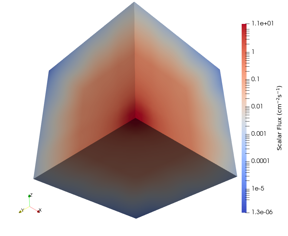
Figure 2: Scalar flux for the first Kobayashi benchmark.
Plotting the post-processed results from the three LineValueSamplers results in Figure 5, Figure 6, and Figure 7.
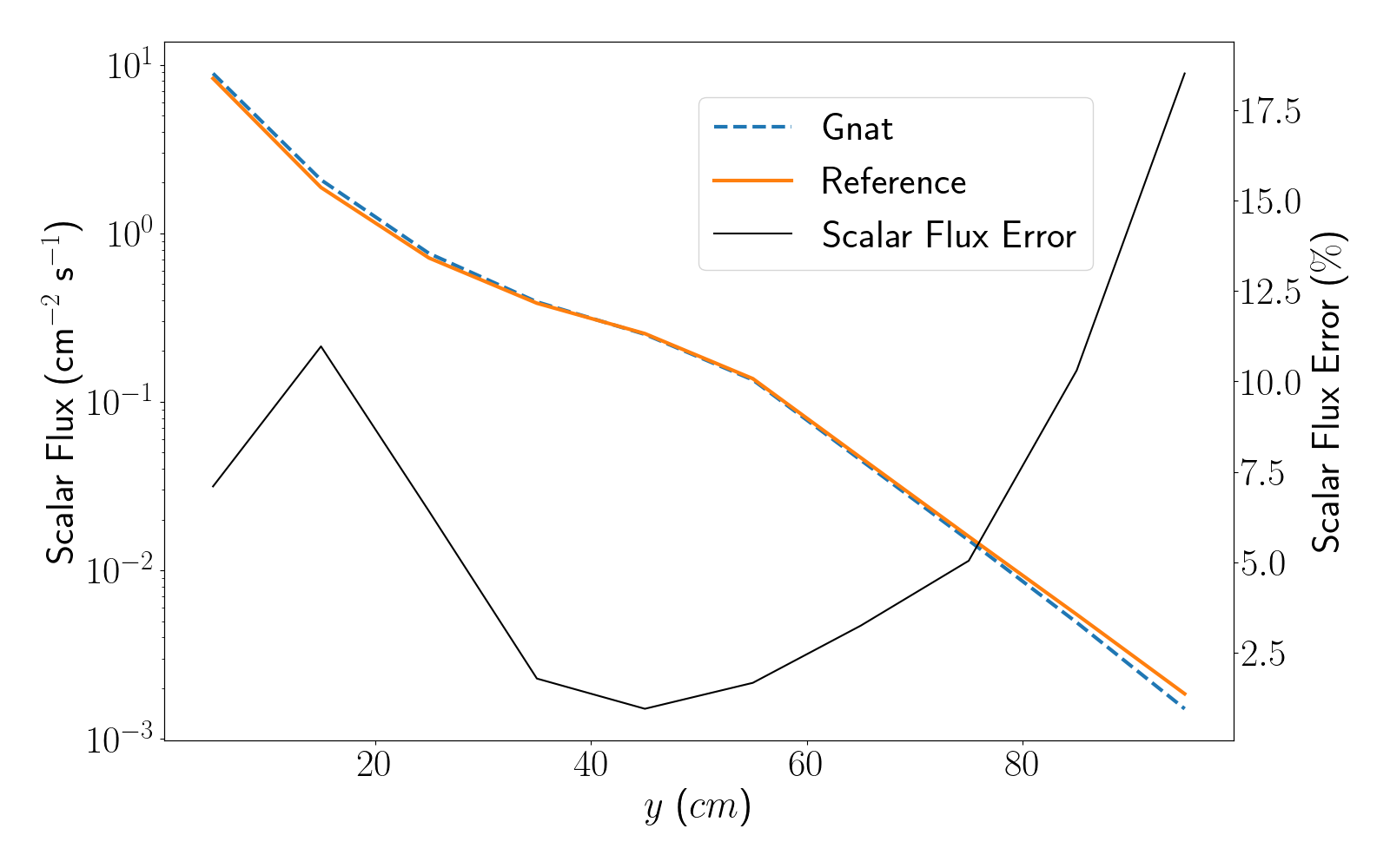
Figure 5: Scalar flux plotted along line A for the first Kobayashi benchmark.
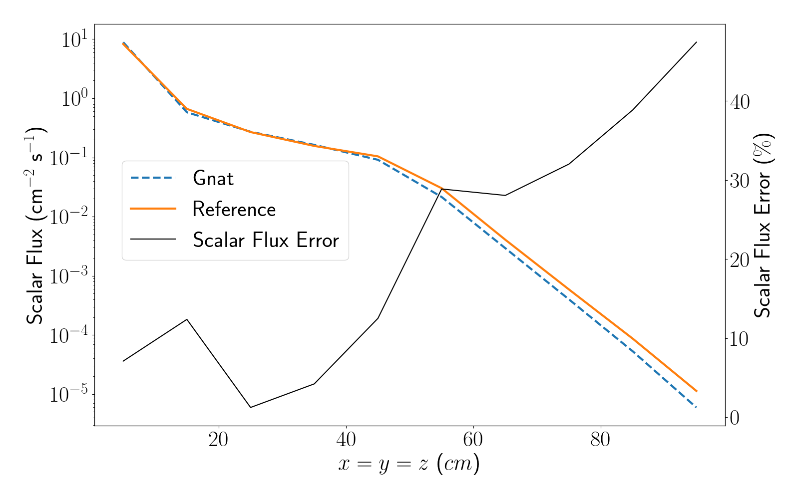
Figure 6: Scalar flux plotted along line B for the first Kobayashi benchmark.
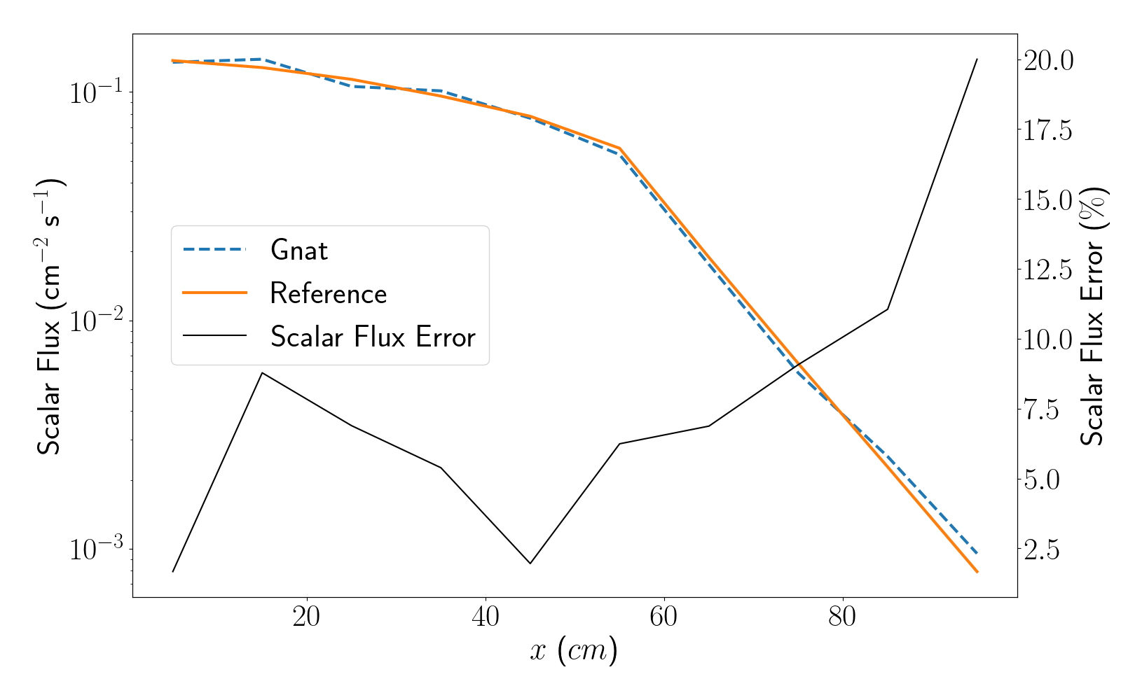
Figure 7: Scalar flux plotted along line C for the first Kobayashi benchmark.
We can clearly see the impact of ray effects from the limited number of samples in the angular quadrature set, alongside the imapct of the coarse spatial discretization which manifest in oscillations in the scalar flux. These will be come more pronounced in the following sections, where the straight duct and dog-legged duct problems are modelled.
Straight Duct
The second Kobayashi benchmark problem consists of a cubic volume source with one corner centered on the origin. It is surrounded by a shield that is thick along the positive y direction and thick along the x and z direction. The long component of the shield is penetrated by a duct with a square cross section, yielding a long streaming path. The geometry of this problem can be found in Figure 3. Similar to the first benchmark problem, three sides use reflective boundary conditions while the remaining three sides use vacuum boundaries.
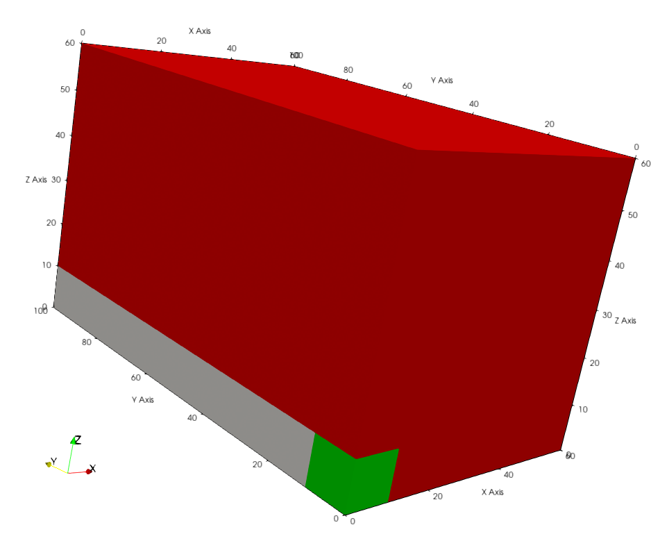
Figure 3: Geometry of the second Kobayashi problem. Green: source. White: near-void. Red: shield.
There are two differences between the previously modelled cubic shield problem and the straight duct problem. The first is the definition of the mesh where dx, dy, and dz are modified to change the configuration of the geometry. ix, iy, and iz are then changed to maintain element intervals. Finally, the blocks are remapped to capture the material changes. The changes to the mesh can be found below.
[Mesh]
  [domain]
    type = CartesianMeshGenerator<<<{"description": "This CartesianMeshGenerator creates a non-uniform Cartesian mesh."}>>>
    dim<<<{"description": "The dimension of the mesh to be generated"}>>> = 3
    dx<<<{"description": "Intervals in the X direction"}>>> = '10 50'
    dy<<<{"description": "Intervals in the Y direction (required when dim>1 otherwise ignored)"}>>> = '10 90'
    dz<<<{"description": "Intervals in the Z direction (required when dim>2 otherwise ignored)"}>>> = '10 50'
    ix<<<{"description": "Number of grids in all intervals in the X direction (default to all one)"}>>> = '1 5'
    iy<<<{"description": "Number of grids in all intervals in the Y direction (default to all one)"}>>> = '1 9'
    iz<<<{"description": "Number of grids in all intervals in the Z direction (default to all one)"}>>> = '1 5'
    subdomain_id<<<{"description": "Block IDs (default to all zero)"}>>> = '
    2 1
    0 1

    1 1
    1 1'
  []
  uniform_refine<<<{"description": "Specify the level of uniform refinement applied to the initial mesh"}>>> = 1
[]The second change to the input file is the LineValueSamplers we use to post-process the solution. Line_A is modified such that it plots down the length of the duct and Line_B is modified such that it plots from the centerline of the duct into the shield at the edge of the domain. The new VectorPostprocessors can be found below.
[VectorPostprocessors]
  [Line_A]
    type = LineValueSampler<<<{"description": "Samples variable(s) along a specified line"}>>>
    variable<<<{"description": "The names of the variables that this VectorPostprocessor operates on"}>>> = flux_moment_1_0_0
    start_point<<<{"description": "The beginning of the line"}>>> = '5.0 5.0  5.0'
    end_point<<<{"description": "The ending of the line"}>>> = '5.0 95.0 5.0'
    num_points<<<{"description": "The number of points to sample along the line"}>>> = 10
    sort_by<<<{"description": "What to sort the samples by"}>>> = y
  []

  [Line_B]
    type = LineValueSampler<<<{"description": "Samples variable(s) along a specified line"}>>>
    variable<<<{"description": "The names of the variables that this VectorPostprocessor operates on"}>>> = flux_moment_1_0_0
    start_point<<<{"description": "The beginning of the line"}>>> = '5.0  95.0 5.0'
    end_point<<<{"description": "The ending of the line"}>>> = '55.0 95.0 5.0'
    num_points<<<{"description": "The number of points to sample along the line"}>>> = 6
    sort_by<<<{"description": "What to sort the samples by"}>>> = x
  []
[]The second Kobayashi problem can be run with the following:
mpiexec -np 4 gnat-opt -i ./kobayashi_2.i --n-threads=2
The scalar flux calculated by Gnat can be found in Figure 4.
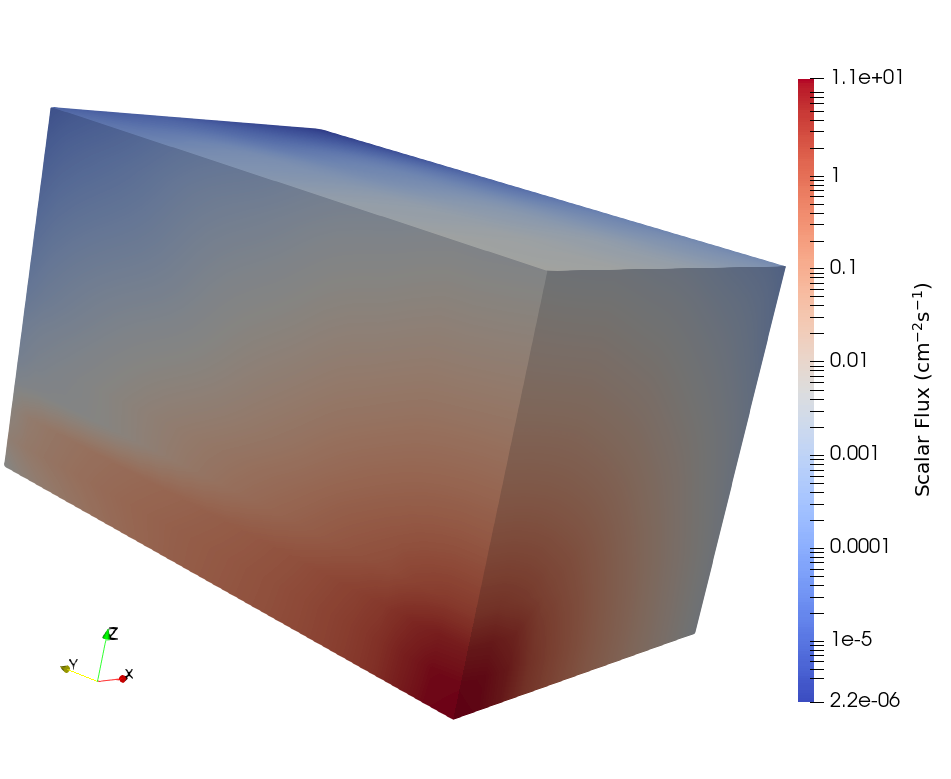
Figure 4: Scalar flux for the second Kobayashi benchmark.
We can really see the ray effects in the solution which are caused by the low order quadrature set. Increasing the number of azimuthal angles per octant (n_azimuthal) would aid in mitigating these ray effects by adding more quadrature directions along the duct, though it would result in a large runtime penalty. The error between the Gnat results and the benchmark along Line_A and Line_B are plotted in Figure 8 and Figure 9. Oscillations caused by the coarse mesh can be seen in Figure 8, and large undershoots in the solution compared to the reference (due to ray effects) can be seen in Figure 9.
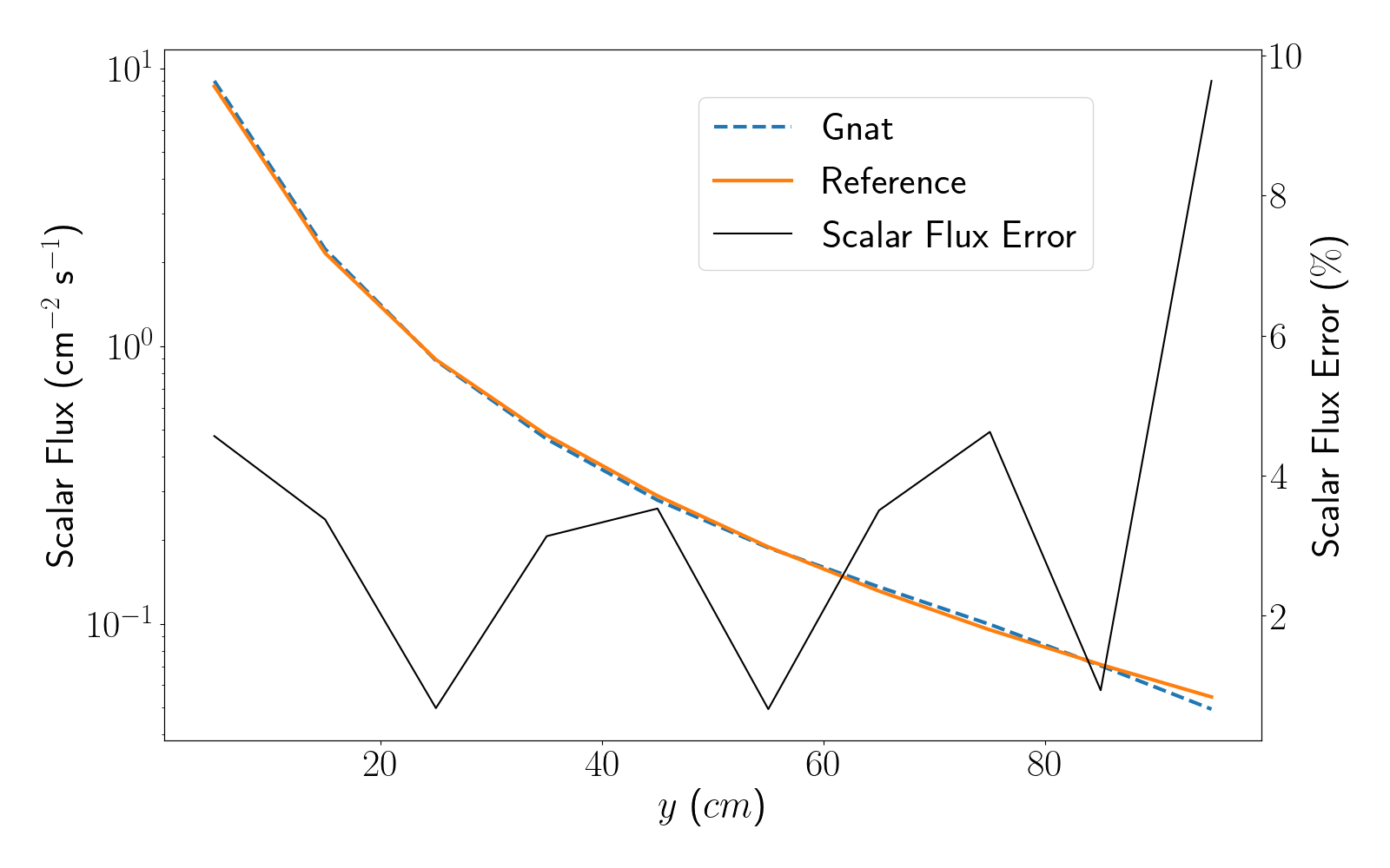
Figure 8: Scalar flux plotted along line A for the second Kobayashi benchmark.
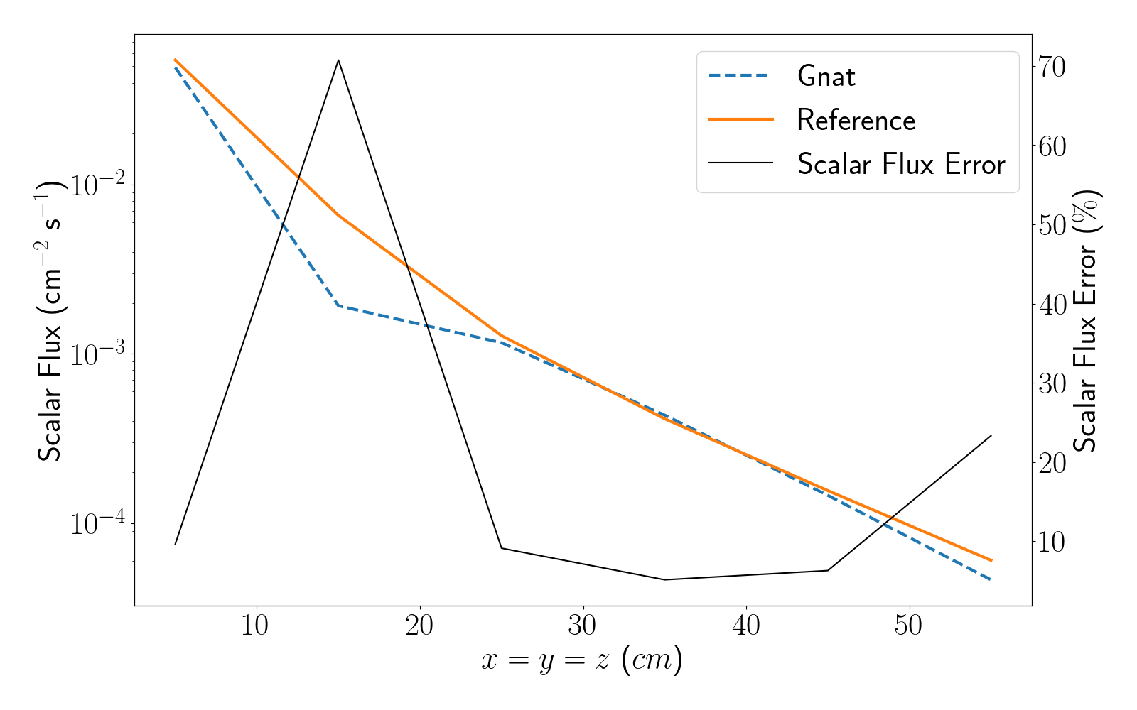
Figure 9: Scalar flux plotted along line B for the second Kobayashi benchmark.
Dog-Legged Duct
The last Kobayashi problem is similar to the second problem, where the only differece is that the duct makes three turns before exiting the shielding medium. The geometry of this problem can be found in Figure 10 and Figure 11.
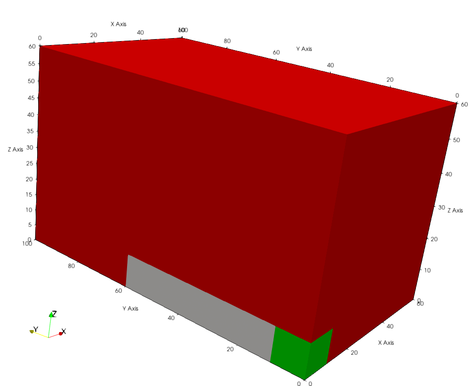
Figure 10: Full geometry of the third Kobayashi problem. Green: source. White: near-void. Red: shield.
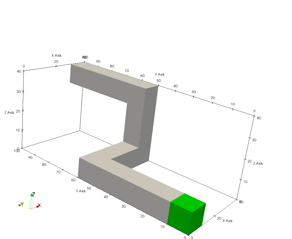
Figure 11: Dog-legged duct in the third Kobayashi problem.
Similar to the straight duct, the only changes we need to make to the input file are to the mesh and the post-processors we add to compare the solution to the reference solution. The [Mesh] block for this problem is substantially more complicated then the first and second problem due to the added heterogeneity; extra slices in dx, dy, and dz are required to model these material changes alongside additional block mappings in subdomain_id. The full mesh block can be found below.
[Mesh]
  [domain]
    type = CartesianMeshGenerator<<<{"description": "This CartesianMeshGenerator creates a non-uniform Cartesian mesh."}>>>
    dim<<<{"description": "The dimension of the mesh to be generated"}>>> = 3
    dx<<<{"description": "Intervals in the X direction"}>>> = '10 20 10 20'
    dy<<<{"description": "Intervals in the Y direction (required when dim>1 otherwise ignored)"}>>> = '10 40 10 40'
    dz<<<{"description": "Intervals in the Z direction (required when dim>2 otherwise ignored)"}>>> = '10 20 10 20'
    ix<<<{"description": "Number of grids in all intervals in the X direction (default to all one)"}>>> = '1 2 1 2'
    iy<<<{"description": "Number of grids in all intervals in the Y direction (default to all one)"}>>> = '1 4 1 4'
    iz<<<{"description": "Number of grids in all intervals in the Z direction (default to all one)"}>>> = '1 2 1 2'
    subdomain_id<<<{"description": "Block IDs (default to all zero)"}>>> = '
    2 1 1 1
    0 1 1 1
    0 0 0 1
    1 1 1 1

    1 1 1 1
    1 1 1 1
    1 1 0 1
    1 1 1 1

    1 1 1 1
    1 1 1 1
    1 1 0 1
    1 1 0 1

    1 1 1 1
    1 1 1 1
    1 1 1 1
    1 1 1 1'
  []
  uniform_refine<<<{"description": "Specify the level of uniform refinement applied to the initial mesh"}>>> = 1
[]When it comes to the changes in post-processors, Line_A plots along the center of the duct (before the first bend). Line_B plots along the interface between the duct and the shield at the first bend. Line_C plots across the duct after the third bend. The modifiications to the LineValueSampler post-processors can be found below.
[VectorPostprocessors]
  [Line_A]
    type = LineValueSampler<<<{"description": "Samples variable(s) along a specified line"}>>>
    variable<<<{"description": "The names of the variables that this VectorPostprocessor operates on"}>>> = flux_moment_1_0_0
    start_point<<<{"description": "The beginning of the line"}>>> = '5.0 5.0  5.0'
    end_point<<<{"description": "The ending of the line"}>>> = '5.0 95.0 5.0'
    num_points<<<{"description": "The number of points to sample along the line"}>>> = 10
    sort_by<<<{"description": "What to sort the samples by"}>>> = y
  []

  [Line_B]
    type = LineValueSampler<<<{"description": "Samples variable(s) along a specified line"}>>>
    variable<<<{"description": "The names of the variables that this VectorPostprocessor operates on"}>>> = flux_moment_1_0_0
    start_point<<<{"description": "The beginning of the line"}>>> = '5.0  55.0 5.0'
    end_point<<<{"description": "The ending of the line"}>>> = '55.0 55.0 5.0'
    num_points<<<{"description": "The number of points to sample along the line"}>>> = 6
    sort_by<<<{"description": "What to sort the samples by"}>>> = x
  []

  [Line_C]
    type = LineValueSampler<<<{"description": "Samples variable(s) along a specified line"}>>>
    variable<<<{"description": "The names of the variables that this VectorPostprocessor operates on"}>>> = flux_moment_1_0_0
    start_point<<<{"description": "The beginning of the line"}>>> = '5.0  95.0 35.0'
    end_point<<<{"description": "The ending of the line"}>>> = '55.0 95.0 35.0'
    num_points<<<{"description": "The number of points to sample along the line"}>>> = 6
    sort_by<<<{"description": "What to sort the samples by"}>>> = x
  []
[]The final Kobayashi problem can be run with the following:
mpiexec -np 4 gnat-opt -i ./kobayashi_3.i --n-threads=2
The scalar flux over the whole problem can be found in Figure 12, and the scalar flux along the duct can be found in Figure 13.
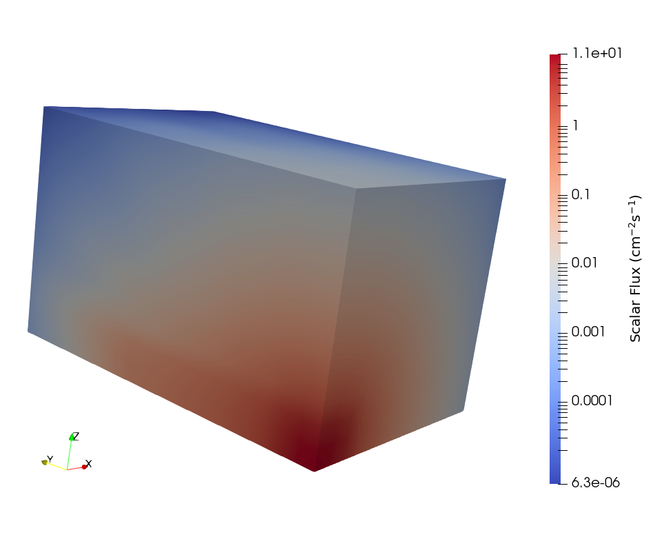
Figure 12: Scalar flux in the third Kobayashi benchmark.
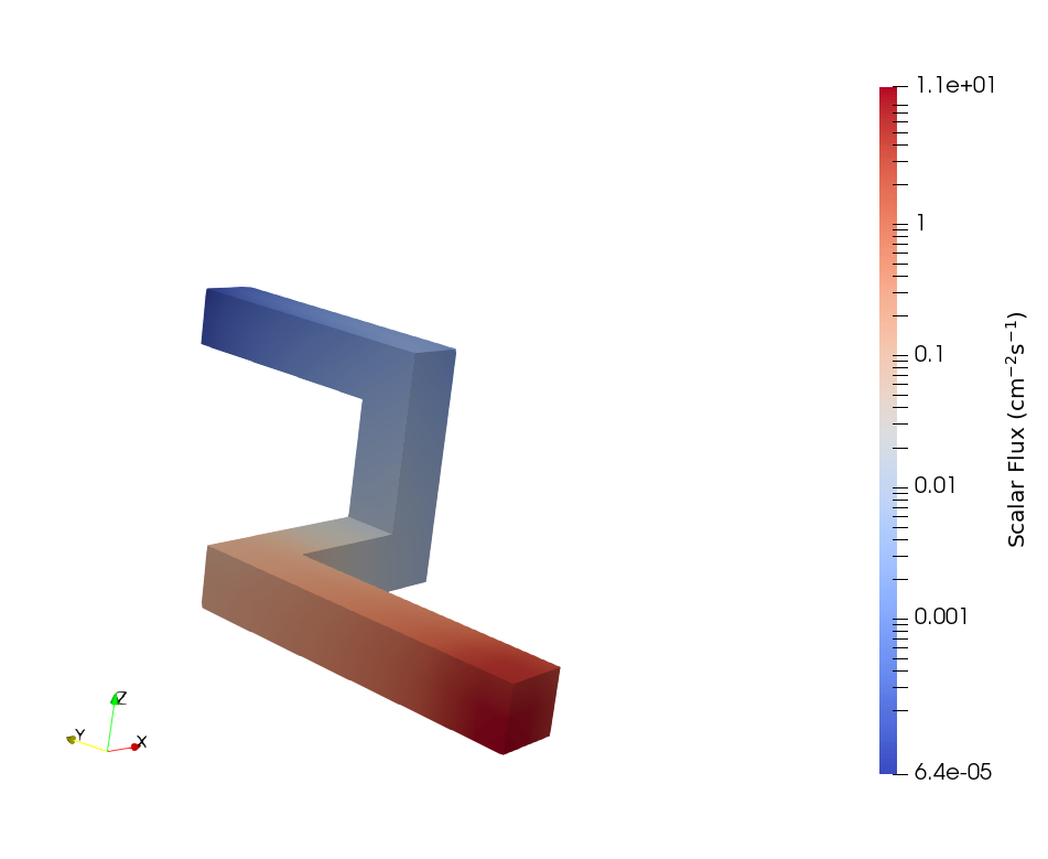
Figure 13: Scalar flux isolated to the dog-legged duct.
The results along each line compared to the reference scalar flux can be found below.
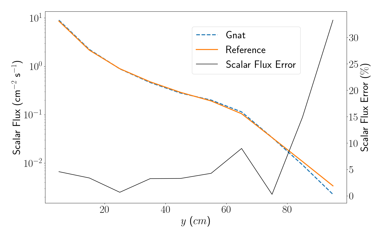
Figure 14: Scalar flux plotted along line A for the first Kobayashi benchmark.
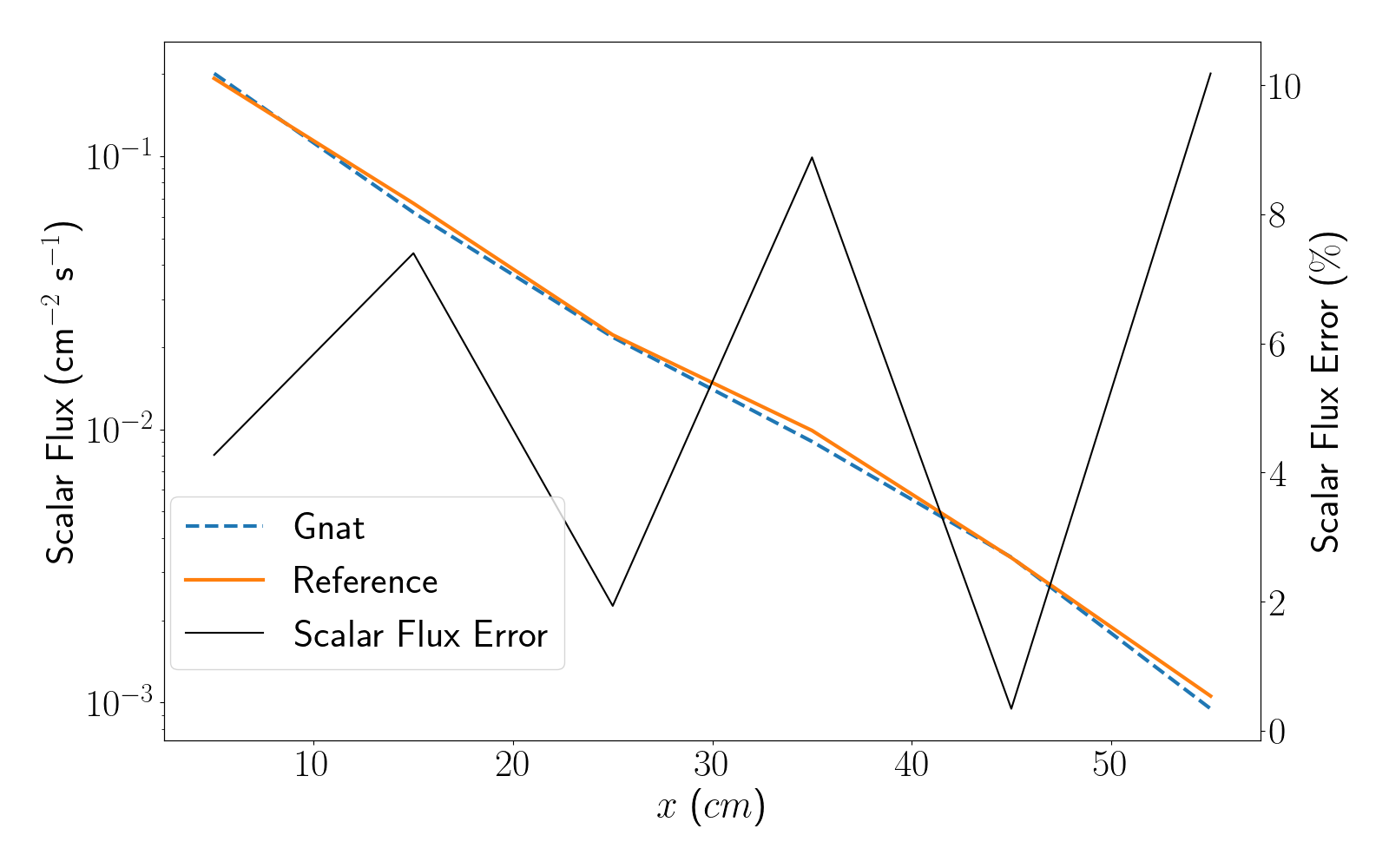
Figure 15: Scalar flux plotted along line B for the first Kobayashi benchmark.
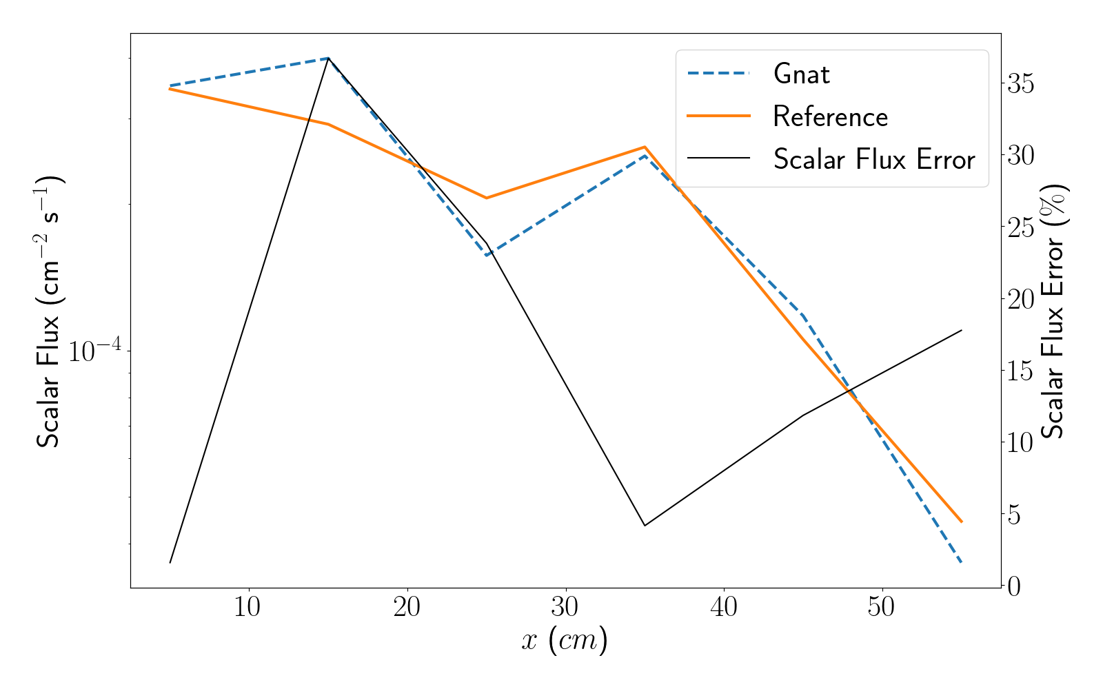
Figure 16: Scalar flux plotted along line C for the first Kobayashi benchmark.
References
- Keisuke Kobayashi, Naoki Sugimura, and Yasunobu Nagaya.
3D Radiation Transport Benchmark Problems and Results for Simple Geometries With Void Region.
Progress in Nuclear Energy (New Series), 39(2):119–144, 2001.
doi:10.1016/S0149-1970(01)00007-5.[BibTeX]