Simple Fixed-Source Problems
In this tutorial, you will learn:
How to model 2D shielding problems in Gnat;
How to provide multi-group material properties;
How to specify point and surface sources.
To access this tutorial,
cd gnat/tutorials/2D_fixed_source
Geometry and Material Properties
This problem is one where an isotropic neutron point source is placed in the middle of a 2D domain that scatters neutrons isotropically and absorbs neutrons. The point source emits at a constant rate of into a single energy group. Vacuum boundaries surround the domain on all four sides and the problem is at steady-state. The material has cm and cm.
The Neutronics Input File
Like any problem which is solved with the finite element method, the first step in using Gnat for neutron transport is to declare a mesh. For a simple case like this one the built-in mesh generators in Moose can be used:
[Mesh]
  [domain]
    type = CartesianMeshGenerator<<<{"description": "This CartesianMeshGenerator creates a non-uniform Cartesian mesh."}>>>
    dim<<<{"description": "The dimension of the mesh to be generated"}>>> = 2
    dx<<<{"description": "Intervals in the X direction"}>>> = 10
    dy<<<{"description": "Intervals in the Y direction (required when dim>1 otherwise ignored)"}>>> = 10
    ix<<<{"description": "Number of grids in all intervals in the X direction (default to all one)"}>>> = 101
    iy<<<{"description": "Number of grids in all intervals in the Y direction (default to all one)"}>>> = 101
  []
[]The CartesianMeshGenerator object generates simple cartesian meshes in 1D, 2D or 3D. dim = 2 is set to let the mesh generator know that a 2D cartesian mesh is required. dx = 10 and dy = 10 set the size of the mesh to 10 cm in both x and y. Finally, ix = 100 and iy = 100 indicate that the mesh should be subdivided into 100 elements along both the x and y axis. The result is shown in Figure 1:
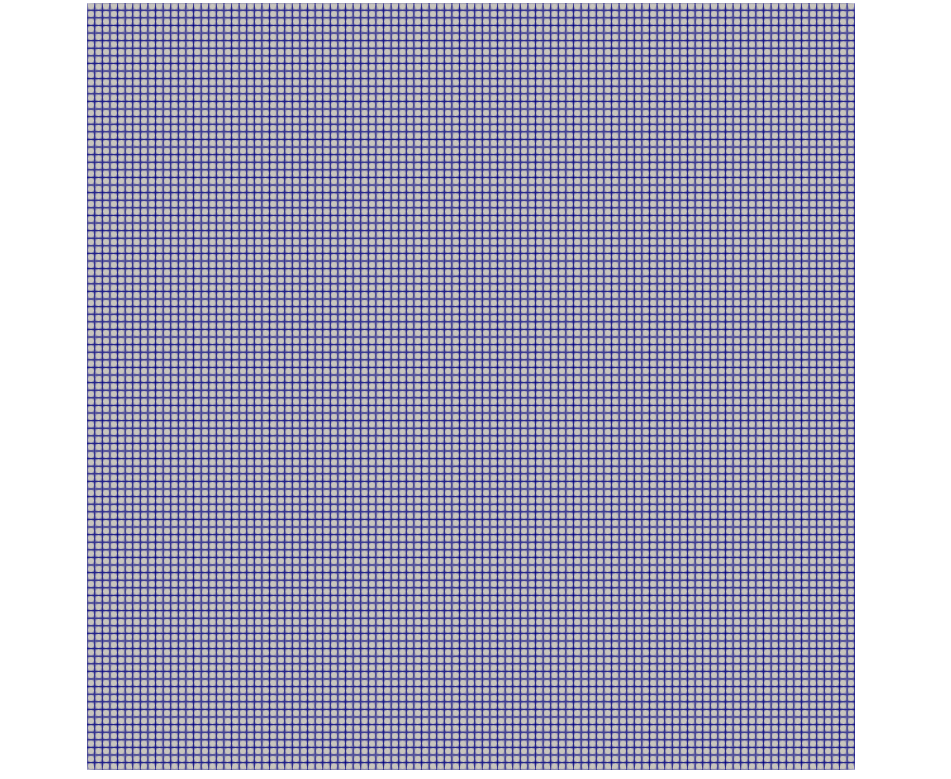
Figure 1: 2D cartesian mesh for the 2D point source problem.
The next step in solving radiation transport problems is to declare a TransportSystem block. This is short-cut syntax that sets up all of the kernels and variables necessary for transport calculations along many directions for many energy groups, which minimizes the length of your Gnat input file.
[TransportSystems<<<{"href": "../syntax/TransportSystems/index.html"}>>>]
  [Neutron]
    num_groups<<<{"description": "The number of spectral energy groups in the problem."}>>> = 1
    max_anisotropy<<<{"description": "The maximum degree of anisotropy to evaluate. Defaults to 0 for isotropic scattering."}>>> = 0
    scheme<<<{"description": "The discretization and stabilization scheme for the transport equation."}>>> = saaf_cfem
    particle_type<<<{"description": "The type of particle to be consuming material property data."}>>> = neutron

    order<<<{"description": "Specifies the order of the FE shape function to use for this variable (additional orders not listed are allowed)."}>>> = FIRST
    family<<<{"description": "Specifies the family of FE shape functions to use for this variable."}>>> = LAGRANGE

    n_azimuthal<<<{"description": "Number of Chebyshev azimuthal quadrature points in a single octant of the unit sphere. Defaults to 3."}>>> = 2
    n_polar<<<{"description": "Number of Legendre polar quadrature points in a single octant of the unit sphere. Defaults to 3."}>>> = 2

    vacuum_boundaries<<<{"description": "The boundaries to apply vacuum boundary conditions."}>>> = 'left right top bottom'

    point_source_locations<<<{"description": "The locations of all isotropic point sources in the problem space."}>>> = '5.0 5.0 0.0'
    point_source_moments<<<{"description": "A double vector containing a list of external source moments for all point particle sources. The external vector should correspond with the order of 'point_source_locations'."}>>> = '1e3'
    point_source_anisotropies<<<{"description": "The anisotropies of the point sources. The vector should correspond with the order of 'point_source_locations'"}>>> = '0'
    scale_sources<<<{"description": "If the external fixed sources should be scaled such that each source moment is divided by the maximum source moment."}>>> = true
  []
[]To start, num_groups = 1 specifies that the transport simulation should only consider a single neutron group although more can be specified at the cost of increased computational complexity. max_anisotropy = 0 tells the transport simulation to only evaluate the 0th-order moment of the angular flux, which is more than enough for this case as scattering is isotropic. scheme = saaf_cfem states that the self-adjoint angular flux stabilization scheme is requested. In accordance with that choice, continuous basis functions in the form of first-order (order = FIRST) Lagrange (family = LAGRANGE) functions are used. The number of angular directions are specified with n_azimuthal = 2 and n_polar = 2, and vacuum boundaries are specified for all sides with vacuum_boundaries = 'left right top bottom'. Finally, the point source is specified with a location at (5.0, 5.0, 5.0) with an emission intensity of 1000 n/s emitting into the single energy group. In addition to specifying the point source, we also set scale_sources = true which divides all source moments by the largest moment value. This rescales the fixed source problem such that the largest source moment is unity, improving the stability of the finite element solve.
Next, the material properties of the domain must be specified. Gnat does this through a system implemented for transport problems known as TransportMaterials:
[TransportMaterials<<<{"href": "../syntax/TransportMaterials/index.html"}>>>]
  [Domain]
    type = ConstantTransportMaterial<<<{"description": "Provides the particle group velocity ($v_{g}$), particle group total cross-section ($\\Sigma_{a,g}$), and the scattering cross-section moments ($\\Sigma_{s, g', g, l}$) for transport problems. If no scattering cross-section moments are provided, the material initializes all moments to 0. The properties must be listed in decreasing order by energy.", "href": "../source/materials/ConstantTransportMaterial.html"}>>>
    transport_system<<<{"description": "Name of the transport system which will consume the provided material properties. If one is not provided the first transport system will be used."}>>> = Neutron
    anisotropy<<<{"description": "The scattering anisotropy of the medium."}>>> = 0
    group_total<<<{"description": "The macroscopic particle total cross-sections for all energy groups."}>>> = 2.0
    group_scattering<<<{"description": "The group-to-group scattering cross-section moments for all energy groups."}>>> = 1.0
  []
[]This declares a constant material which provides enough parameters for a single neutron group. The material provides an isotropic scattering cross section (anisotropy = 0). The material has an total cross section of 2 (group_total = 2.0) and a scattering cross section of 1 (group_scattering = 1.0). transport_system = Neutron links this material to the Neutron transport system previously declared.
The remainder of the input file describes how the problem should be solved:
[Executioner]
  type = Steady
  solve_type = PJFNK
  petsc_options_iname = '-pc_type -pc_hypre_type -ksp_gmres_restart'
  petsc_options_value = ' hypre    boomeramg      10'
  l_max_its = 50
  nl_rel_tol = 1e-12
[]The Executioner block declares the solver parameters and solve type. In this case, type = Steady and the Preconditioned Jacobian-Free Newton Krylov (solve_type = PJFNK) is used. It is recommended that the user employ the PJFNK solver for continuous finite element methods when solving radiation transport problems with the SAAF-CFEM scheme.
The simulation can be executed with the following shell command:
mpiexec -np 2 gnat-opt -i ./2D_point_source.i --n-threads=2
The results of this simple case can be seen below in Figure 2:
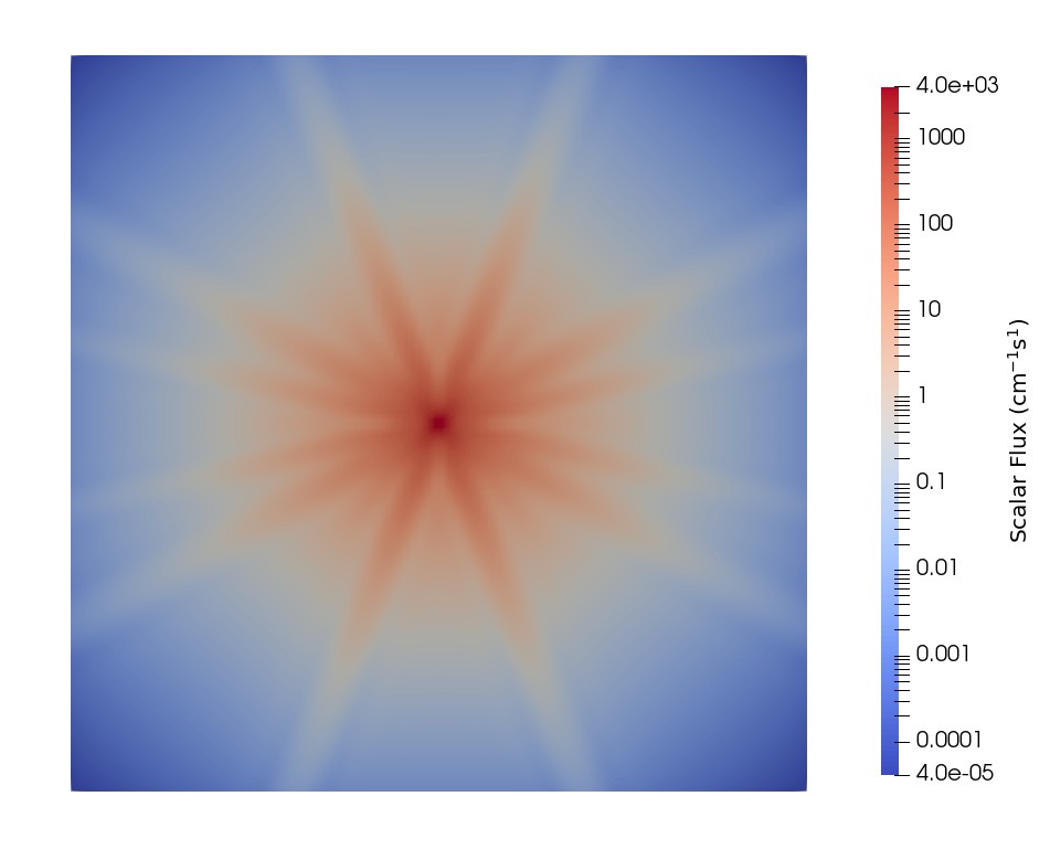
Figure 2: Scalar flux from the 2D point source problem.
We can see the signature disadvantage of the discrete ordiantes method: ray effects. These occur because of the limited angular resolution (four directions per quadrant of the 2D unit sphere) of the chosen discretization compared to the small size of the fixed source. We can attempt to mitigate these ray effects by adding extra directions by specifying n_azimuthal = 10 and n_polar = 10, which results in Figure 3.
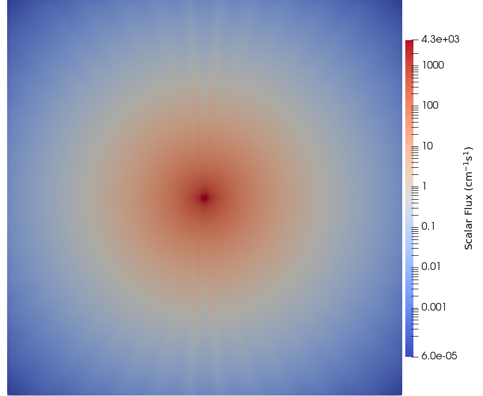
Figure 3: Refined scalar flux from the 2D point source problem.
However, the increased angular fidelity results in a large increase in runtime with diminishing returns. Instead of increasing the number of directions one could instead use an uncollided flux technique, which is discussed in the uncollided flux tutorial.
Adding a Second Energy Group
In this section, we modify the problem to add a second energy group. The modifications made to the transport system can be found below.
[TransportSystems<<<{"href": "../syntax/TransportSystems/index.html"}>>>]
  [Neutron]
    num_groups<<<{"description": "The number of spectral energy groups in the problem."}>>> = 2
    max_anisotropy<<<{"description": "The maximum degree of anisotropy to evaluate. Defaults to 0 for isotropic scattering."}>>> = 0
    scheme<<<{"description": "The discretization and stabilization scheme for the transport equation."}>>> = saaf_cfem
    particle_type<<<{"description": "The type of particle to be consuming material property data."}>>> = neutron

    order<<<{"description": "Specifies the order of the FE shape function to use for this variable (additional orders not listed are allowed)."}>>> = FIRST
    family<<<{"description": "Specifies the family of FE shape functions to use for this variable."}>>> = LAGRANGE

    n_azimuthal<<<{"description": "Number of Chebyshev azimuthal quadrature points in a single octant of the unit sphere. Defaults to 3."}>>> = 2
    n_polar<<<{"description": "Number of Legendre polar quadrature points in a single octant of the unit sphere. Defaults to 3."}>>> = 2

    vacuum_boundaries<<<{"description": "The boundaries to apply vacuum boundary conditions."}>>> = 'left right top bottom'

    point_source_locations<<<{"description": "The locations of all isotropic point sources in the problem space."}>>> = '5.0 5.0 0.0'
    point_source_moments<<<{"description": "A double vector containing a list of external source moments for all point particle sources. The external vector should correspond with the order of 'point_source_locations'."}>>> = '1e3 1.0'
    point_source_anisotropies<<<{"description": "The anisotropies of the point sources. The vector should correspond with the order of 'point_source_locations'"}>>> = '0'
    scale_sources<<<{"description": "If the external fixed sources should be scaled such that each source moment is divided by the maximum source moment."}>>> = true
  []
[]We specify that two energy groups should be added by setting num_groups = 2. We then add a second source moment for the point source with point_source_moments = '1e3 1.0'. The TransportMaterials block then needs to be modified with a new set of group properties.
[TransportMaterials<<<{"href": "../syntax/TransportMaterials/index.html"}>>>]
  [Domain]
    type = ConstantTransportMaterial<<<{"description": "Provides the particle group velocity ($v_{g}$), particle group total cross-section ($\\Sigma_{a,g}$), and the scattering cross-section moments ($\\Sigma_{s, g', g, l}$) for transport problems. If no scattering cross-section moments are provided, the material initializes all moments to 0. The properties must be listed in decreasing order by energy.", "href": "../source/materials/ConstantTransportMaterial.html"}>>>
    transport_system<<<{"description": "Name of the transport system which will consume the provided material properties. If one is not provided the first transport system will be used."}>>> = Neutron
    anisotropy<<<{"description": "The scattering anisotropy of the medium."}>>> = 0
    group_total<<<{"description": "The macroscopic particle total cross-sections for all energy groups."}>>> = '1.0 2.0'
    group_scattering<<<{"description": "The group-to-group scattering cross-section moments for all energy groups."}>>> = '0.4 0.1
                        0.0 2.0'
  []
[]Here, we modify the total cross section such that it's representative of two-group transport in a highly scattering material (such as water). The scattering cross section becomes a scattering matrix with zero thermal upscattering. This modified input deck can be run with:
mpiexec -np 2 gnat-opt -i ./2D_point_source_2_grp.i --n-threads=2
The results for group 1 (fast) can be found in Figure 4, while the results for group 2 (thermal) can be found in Figure 5.
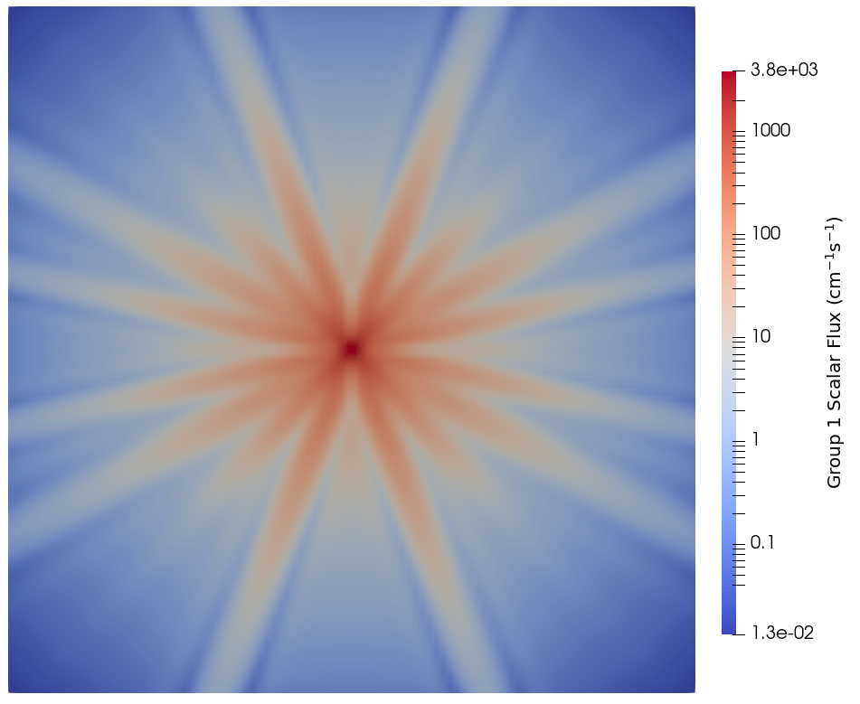
Figure 4: Group 1 scalar flux from the 2D point source problem.
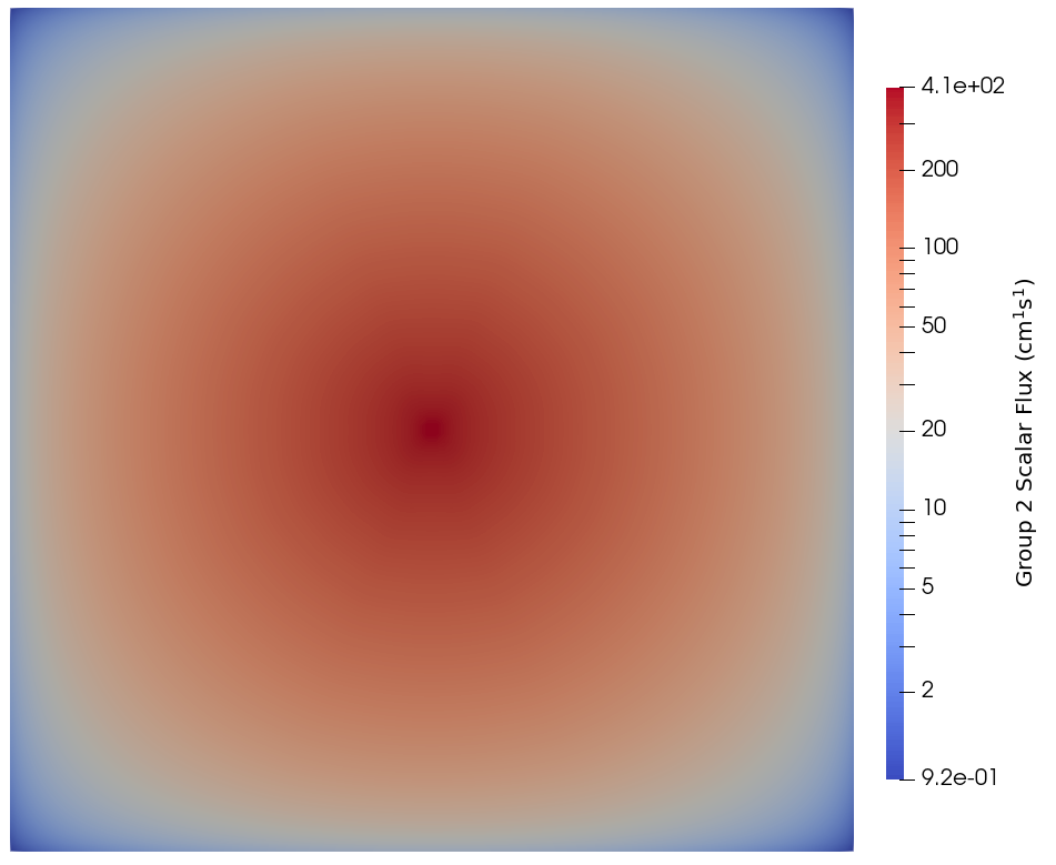
Figure 5: Group 2 scalar flux from the 2D point source problem.
Similar to Figure 2, we can see ray effects in the fast energy group due to the low within-group scattering cross section relative to the total cross section. The effect of fast-to-thermal scattering and the large within-group thermal scattering cross section can be seen in Figure 5, where there are no ray effect even though the point source emits into group two.
Swapping the Point Source for a Surface Source
In this section, we remove the point source and add an isotropic surface source on the top boundary of the domain. This requires a few minor modifications to the TransportSystem.
[TransportSystems<<<{"href": "../syntax/TransportSystems/index.html"}>>>]
  [Neutron]
    num_groups<<<{"description": "The number of spectral energy groups in the problem."}>>> = 2
    max_anisotropy<<<{"description": "The maximum degree of anisotropy to evaluate. Defaults to 0 for isotropic scattering."}>>> = 0
    scheme<<<{"description": "The discretization and stabilization scheme for the transport equation."}>>> = saaf_cfem
    particle_type<<<{"description": "The type of particle to be consuming material property data."}>>> = neutron

    order<<<{"description": "Specifies the order of the FE shape function to use for this variable (additional orders not listed are allowed)."}>>> = FIRST
    family<<<{"description": "Specifies the family of FE shape functions to use for this variable."}>>> = LAGRANGE

    n_azimuthal<<<{"description": "Number of Chebyshev azimuthal quadrature points in a single octant of the unit sphere. Defaults to 3."}>>> = 2
    n_polar<<<{"description": "Number of Legendre polar quadrature points in a single octant of the unit sphere. Defaults to 3."}>>> = 2

    vacuum_boundaries<<<{"description": "The boundaries to apply vacuum boundary conditions."}>>> = 'left right bottom'
    source_boundaries<<<{"description": "The boundaries to apply incoming flux boundary conditions."}>>> = 'top'

    boundary_source_moments<<<{"description": "A double vector containing the external source moments for all boundaries. The exterior vector must correspond with the surface source boundary conditions provided in 'source_boundaries'."}>>> = '1e3 1.0'
    boundary_source_anisotropy<<<{"description": "The degree of anisotropy of the boundary source moments. The exterior vector must correspond with the surface source boundary conditions provided in 'source_boundaries'."}>>> = '0'
    scale_sources<<<{"description": "If the external fixed sources should be scaled such that each source moment is divided by the maximum source moment."}>>> = true
  []
[]point_source_locations is replaced with source_boundaries, which contains the side sets on which we wish to apply the surface source. point_source_moments and point_source_anisotropies are then replaced with their surface source equivalents: boundary_source_moments and boundary_source_anisotropy. This modified input deck can be run with:
mpiexec -np 2 gnat-opt -i ./2D_surface_source_2_grp.i --n-threads=2
The results for group 1 (fast) can be found in Figure 6, while the results for group 2 (thermal) can be found in Figure 7.
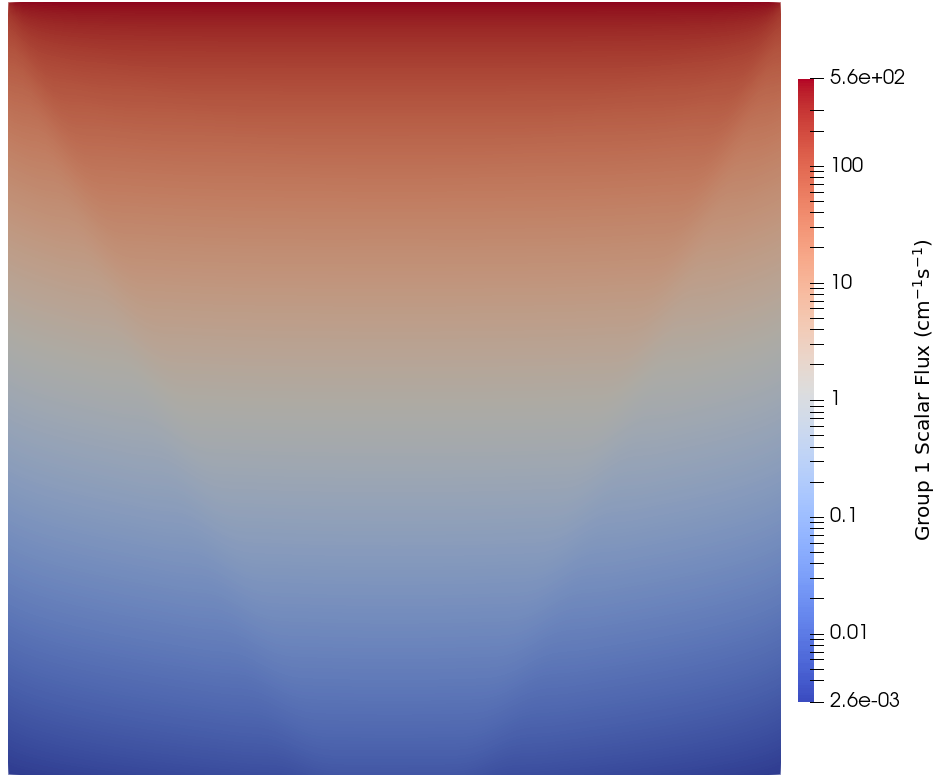
Figure 6: Group 1 scalar flux from the 2D surface source problem.
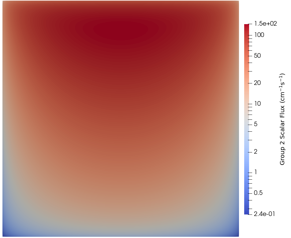
Figure 7: Group 2 scalar flux from the 2D surface source problem.