The Reed Benchmark Problem
In this tutorial, you will learn:
The basics of setting up a neutron transport problems in Gnat;
How to model the 1D Reed benchmark problem.
To access this tutorial,
cd gnat/tutorials/1D_reed_sn
Geometry and Material Properties
The Reed problem is a classic benchmark proposed in Reed (1971) which is used to test the accuracy of space-angle discretization schemes, and serves as the "hello world" in the radiation transport community. It consists of a 1D slab with five distinct material regions, which can be found below in Table 1.
Table 1: Material properties for the 1D Reed problem.
| ID | Region | () | () | () |
|---|---|---|---|---|
| 1 | 50.0 | 0.0 | 50.0 | |
| 2 | 5.0 | 0.0 | 50.0 | |
| 3 | 0.0 | 0.0 | 50.0 | |
| 4 | 1.0 | 0.9 | 1.0 | |
| 5 | 1.0 | 0.9 | 0.0 |
The slab is arranged such that the left boundary is a reflective (symmetry) boundary, and the right boundary is a vacuum boundary condition.
The Neutronics Input File
Like any problem which is solved with the finite element method, the first step when using Gnat for neutron transport is to declare a mesh. The Reed benchmark is incredibly simple, so we can use MOOSE's built-in CartesianMeshGenerator:
[Mesh]
  [domain]
    type = CartesianMeshGenerator<<<{"description": "This CartesianMeshGenerator creates a non-uniform Cartesian mesh."}>>>
    dim<<<{"description": "The dimension of the mesh to be generated"}>>> = 1
    dx<<<{"description": "Intervals in the X direction"}>>> = '2.0 1.0 2.0 1.0 2.0'
    ix<<<{"description": "Number of grids in all intervals in the X direction (default to all one)"}>>> = '4 2 4 2 4'
    subdomain_id<<<{"description": "Block IDs (default to all zero)"}>>> = '0 1 2 3 4'
  []
[]Here, we specify the mesh should be 1D with dim = 1. This is followed by the unique spatial regions in dx. Afterwards, the number of subdivisions per region are specified in ix - initially set such that that each element is cm long. Finally, we set the unique material regions in blocks. This mesh generator automatically generates side sets called left and right, which we can use to apply boundary conditions.
The next step is to set up the radiation transport problem. If we were to do this with MOOSE's default input syntax, we would need to add variables and kernels for each direction and each energy group. This would be incredibly tedious, so Gnat provides input syntax to automate this process with the TransportSystems block:
[TransportSystems<<<{"href": "../syntax/TransportSystems/index.html"}>>>]
  [Neutron]
    num_groups<<<{"description": "The number of spectral energy groups in the problem."}>>> = 1
    scheme<<<{"description": "The discretization and stabilization scheme for the transport equation."}>>> = saaf_cfem
    particle_type<<<{"description": "The type of particle to be consuming material property data."}>>> = neutron

    order<<<{"description": "Specifies the order of the FE shape function to use for this variable (additional orders not listed are allowed)."}>>> = FIRST
    family<<<{"description": "Specifies the family of FE shape functions to use for this variable."}>>> = LAGRANGE

    n_polar<<<{"description": "Number of Legendre polar quadrature points in a single octant of the unit sphere. Defaults to 3."}>>> = 10

    vacuum_boundaries<<<{"description": "The boundaries to apply vacuum boundary conditions."}>>> = 'right'
    reflective_boundaries<<<{"description": "The boundaries to apply reflective boundary conditions."}>>> = 'left'

    volumetric_source_blocks<<<{"description": "The list of blocks (ids or names) that host a volumetric source."}>>> = '0 3'
    volumetric_source_moments<<<{"description": "A double vector containing a list of external source moments for all volumetric particle sources. The external vector should correspond with the order of 'volumetric_source_blocks'."}>>> = '50.0; 1.0'
    volumetric_source_anisotropies<<<{"description": "The anisotropies of the volumetric sources. The vector should correspond with the order of 'volumetric_source_blocks'"}>>> = '0 0'
  []
[]Here, we create a "transport system" named Neutron. We specify that it should be mono-energetic with num_groups = 1, and that it should use the SAAF-CFEM-SN scheme for discretizing the transport equation (scheme = saaf_cfem). We then specify that particle_type = neutron, indicating that we want to add kernels relevant to neutrons. For the purposes of the Reed benchmark problem, one could also specify particle_type = photon. We then move into discretization parameters, specifying that linear Lagrange basis functions should be used and that the angular quadrature set should use 10 polar angles per half of the unit interval. Afterwards, we set vacuum_boundaries = right and reflective_boundaries = left to apply our boundary conditions. Finally, we add volumetric sources to block 0 (region 1) and block 3 (region 4). These sources are isotropic, and so we set anisotropy to zero for both. We note that volumetric_source_moments is a double vector, where the first index corresponds to the source block, and the second index is the source coefficients for a spherical harmonics expansion in angle for all energy groups.
After spetting up our transport system, we proceed to add the material properties necessary for a transport calculation. This is done with the TransportMaterials block, which links the added material properties to a transport system.
[TransportMaterials<<<{"href": "../syntax/TransportMaterials/index.html"}>>>]
  [One]
    type = ConstantTransportMaterial<<<{"description": "Provides the particle group velocity ($v_{g}$), particle group total cross-section ($\\Sigma_{a,g}$), and the scattering cross-section moments ($\\Sigma_{s, g', g, l}$) for transport problems. If no scattering cross-section moments are provided, the material initializes all moments to 0. The properties must be listed in decreasing order by energy.", "href": "../source/materials/ConstantTransportMaterial.html"}>>>
    transport_system<<<{"description": "Name of the transport system which will consume the provided material properties. If one is not provided the first transport system will be used."}>>> = Neutron
    group_total<<<{"description": "The macroscopic particle total cross-sections for all energy groups."}>>> = '50.0'
    group_scattering<<<{"description": "The group-to-group scattering cross-section moments for all energy groups."}>>> = '0.0'
    block<<<{"description": "The list of blocks (ids or names) that this object will be applied"}>>> = '0'
  []
  [Two]
    type = ConstantTransportMaterial<<<{"description": "Provides the particle group velocity ($v_{g}$), particle group total cross-section ($\\Sigma_{a,g}$), and the scattering cross-section moments ($\\Sigma_{s, g', g, l}$) for transport problems. If no scattering cross-section moments are provided, the material initializes all moments to 0. The properties must be listed in decreasing order by energy.", "href": "../source/materials/ConstantTransportMaterial.html"}>>>
    transport_system<<<{"description": "Name of the transport system which will consume the provided material properties. If one is not provided the first transport system will be used."}>>> = Neutron
    group_total<<<{"description": "The macroscopic particle total cross-sections for all energy groups."}>>> = '5.0'
    group_scattering<<<{"description": "The group-to-group scattering cross-section moments for all energy groups."}>>> = '0.0'
    block<<<{"description": "The list of blocks (ids or names) that this object will be applied"}>>> = '1'
  []
  [Three]
    type = ConstantTransportMaterial<<<{"description": "Provides the particle group velocity ($v_{g}$), particle group total cross-section ($\\Sigma_{a,g}$), and the scattering cross-section moments ($\\Sigma_{s, g', g, l}$) for transport problems. If no scattering cross-section moments are provided, the material initializes all moments to 0. The properties must be listed in decreasing order by energy.", "href": "../source/materials/ConstantTransportMaterial.html"}>>>
    transport_system<<<{"description": "Name of the transport system which will consume the provided material properties. If one is not provided the first transport system will be used."}>>> = Neutron
    group_total<<<{"description": "The macroscopic particle total cross-sections for all energy groups."}>>> = '0.0'
    group_scattering<<<{"description": "The group-to-group scattering cross-section moments for all energy groups."}>>> = '0.0'
    block<<<{"description": "The list of blocks (ids or names) that this object will be applied"}>>> = '2'
  []
  [Four]
    type = ConstantTransportMaterial<<<{"description": "Provides the particle group velocity ($v_{g}$), particle group total cross-section ($\\Sigma_{a,g}$), and the scattering cross-section moments ($\\Sigma_{s, g', g, l}$) for transport problems. If no scattering cross-section moments are provided, the material initializes all moments to 0. The properties must be listed in decreasing order by energy.", "href": "../source/materials/ConstantTransportMaterial.html"}>>>
    transport_system<<<{"description": "Name of the transport system which will consume the provided material properties. If one is not provided the first transport system will be used."}>>> = Neutron
    group_total<<<{"description": "The macroscopic particle total cross-sections for all energy groups."}>>> = '1.0'
    group_scattering<<<{"description": "The group-to-group scattering cross-section moments for all energy groups."}>>> = '0.9'
    block<<<{"description": "The list of blocks (ids or names) that this object will be applied"}>>> = '3'
  []
  [Five]
    type = ConstantTransportMaterial<<<{"description": "Provides the particle group velocity ($v_{g}$), particle group total cross-section ($\\Sigma_{a,g}$), and the scattering cross-section moments ($\\Sigma_{s, g', g, l}$) for transport problems. If no scattering cross-section moments are provided, the material initializes all moments to 0. The properties must be listed in decreasing order by energy.", "href": "../source/materials/ConstantTransportMaterial.html"}>>>
    transport_system<<<{"description": "Name of the transport system which will consume the provided material properties. If one is not provided the first transport system will be used."}>>> = Neutron
    group_total<<<{"description": "The macroscopic particle total cross-sections for all energy groups."}>>> = '1.0'
    group_scattering<<<{"description": "The group-to-group scattering cross-section moments for all energy groups."}>>> = '0.9'
    block<<<{"description": "The list of blocks (ids or names) that this object will be applied"}>>> = '4'
  []
[]We add a ConstantTransportMaterial for each region, which allows for the specification of constant material properties in a spatial region. transport_system = Neutron links these properties to the transport system we created earlier, and block specifies the subdomain that the materials should be applied over. group_total is equivalent to (the group-wise total cross section), and group_scattering is equivalent to (the group-wise scattering matrix).
The final components of a Gnat input file are the specification of the execution type (Steady vs Transient vs Eigen) and the execution settings. The Reed problem is a fixed source problem, so we select type = Steady in the Executioner block. We chose a PJFNK solver to avoid the need to form the full system Jacobian matrix which results in substantial memory savings. The remaining settings improve the convergence rate of the PJFNK solver. These execution settings can be found in the code block below.
[Executioner]
  type = Steady
  solve_type = PJFNK
  petsc_options_iname = '-ksp_gmres_restart'
  petsc_options_value = ' 100'
[]In addition to specifying execution settings, we also add a vector post-processor to plot the solution along the 1D mesh and specify that we want both Exodus and CSV output. This allows us to visualize our results.
[VectorPostprocessors]
  [scalar_flux]
    type = LineValueSampler<<<{"description": "Samples variable(s) along a specified line"}>>>
    sort_by<<<{"description": "What to sort the samples by"}>>> = x
    variable<<<{"description": "The names of the variables that this VectorPostprocessor operates on"}>>> = 'flux_moment_1_0_0'
    start_point<<<{"description": "The beginning of the line"}>>> = '0 0 0'
    end_point<<<{"description": "The ending of the line"}>>> = '8 0 0'
    num_points<<<{"description": "The number of points to sample along the line"}>>> = 1000
  []
[]

[Outputs]
  exodus<<<{"description": "Output the results using the default settings for Exodus output."}>>> = true
  csv<<<{"description": "Output the scalar variable and postprocessors to a *.csv file using the default CSV output."}>>> = true
  execute_on<<<{"description": "The list of flag(s) indicating when this object should be executed. For a description of each flag, see https://mooseframework.inl.gov/source/interfaces/SetupInterface.html."}>>> = 'TIMESTEP_END'
[]Execution and Post-Processing
To run the Reed benchmark problem,
gnat-opt -i 1D_reed.i
Congratulations, you've successfully run your first transport problem with Gnat! We can plot the output from the vector post-processor (1D_reed_out_scalar_flux_0001.csv) in Python, which results in Figure 1.
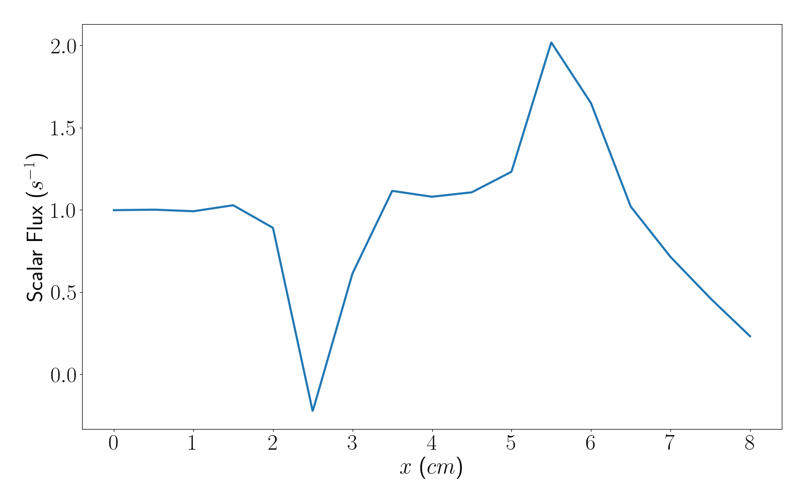
Figure 1: Flux from the Reed benchmark with no mesh subdivisions.
Our flux solution is quite coarse, indicating that added mesh refinement is required to resolve the spatial gradients. The mesh can be refined by adding the following command line arguement when running the input file:
gnat-opt -i 1D_reed.i Mesh/uniform_refine=5
We can see that this took slightly longer to run then the coarse calculations (not by much as 1D transport problems are quite fast); the results of which can be found in Figure 2.
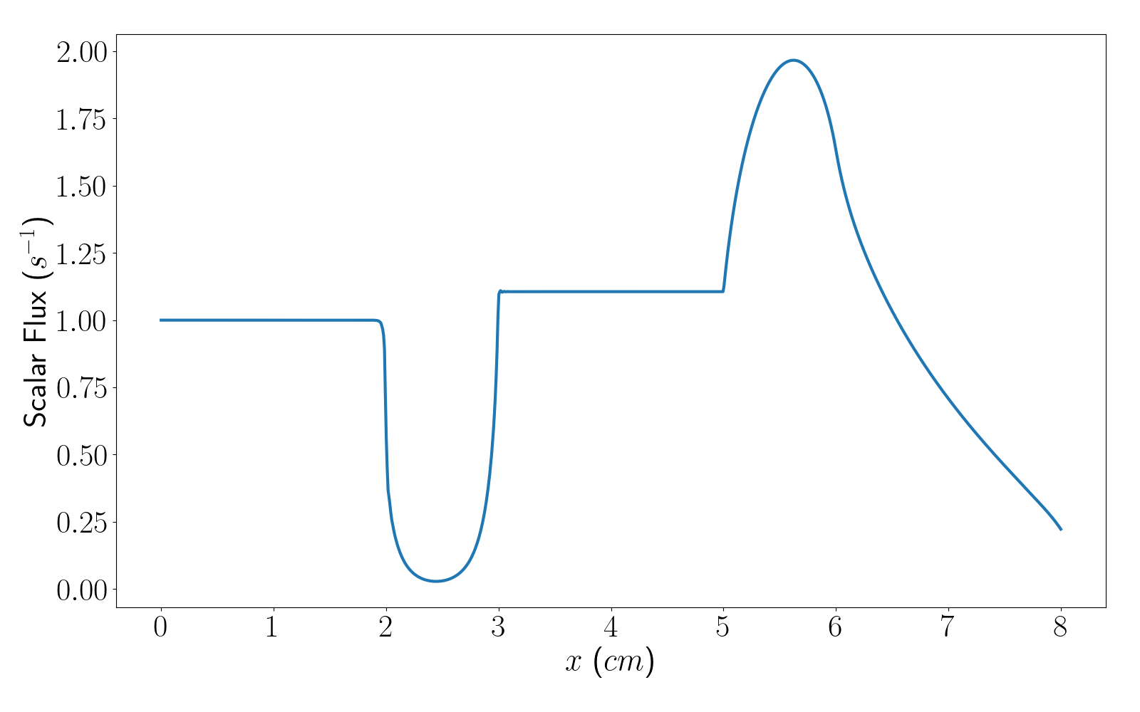
Figure 2: Flux from the Reed benchmark with 5 uniform subdivisions.
References
- William H. Reed.
New Difference Schemes for the Neutron Transport Equation.
Nuclear Science and Engineering, 46(2):309–314, 1971.
doi:10.13182/NSE46-309.[BibTeX]